Dotchart nach Cleveland

Alternativ zum Barplot, wenn Mittelwerte oder Mediane gruppenweise dargestellt werden sollen:

dotchart( tapply( ToothGrowth$len,  list(ToothGrowth$supp, ToothGrowth$dose), mean )
  , main="Guinea Pigs' Tooth Growth", cex=0.8
  , xlab="Vitamin C dose", ylab="tooth length")

Stripchart

Als Alternative zum Boxplot mit wenigen Datenpunkten eignet sich der Stripchart.

stripchart( len ~ dose, data=ToothGrowth, method="jitter", vertical=T
  , subset = supp == "VC", col="blue", main="Guinea Pigs' Tooth Growth"
  , xlab="Vitamin C dose", ylab="tooth length")

stripchart( len ~ dose, data=ToothGrowth, method="jitter", vertical=T
  , subset = supp == "OJ", col="red", add=T)

Grösse des Plot-Fensters bestimmen

Die Grösse des Plot-Fensters kann mit windows() festgelegt werden. Das Grafikfenster wird mit dev.off() wieder geschlossen.

windows(width=10, height=5)
plot( 1:5 )
dev.off()

Selektieren von Listenelementen

Listenelemente können systematisch mit lapply( list, "[", element ) extrahiert werden.

d.frm <- data.frame( id_name=c("1-Max","2-Maria","3-Steven","4-Jane"))

# split into list
lst <- strsplit( x=as.character(d.frm$id_name), split="-" )
# get first elements out of list
d.frm$id <- as.integer( unlist( lapply( lst, "[", 1) ))
d.frm$name <- unlist( lapply( lst, "[", 2) )

d.frm
   id_name   name id
1    1-Max    Max  1
2  2-Maria  Maria  2
3 3-Steven Steven  3
4   4-Jane   Jane  4

str(d.frm)
'data.frame':   4 obs. of  3 variables:
 $ id_name: Factor w/ 4 levels "1-Max","2-Maria",..: 1 2 3 4
 $ name   : chr  "Max" "Maria" "Steven" "Jane"
 $ id     : int  1 2 3 4

Reduce margin between plot region and axes with xaxs, yaxs

# get some data
x.i <- seq(0,1,length=5); y.i <- c( 0,0.1,0.2,0.8,1)
par(mfrow=c(1,2))

plot( y=y.i, x=x.i, type="s", panel.before=grid())
symbols( x=0, y=0, circles=0.12, inches=F, add=T, xpd=T, bg=rgb(0,0,1,0.2) )

plot( y=y.i, x=x.i, type="s", xaxs="i", yaxs="i")
grid(); box()
symbols( x=0, y=0, circles=0.12, inches=F, add=T, xpd=T, bg=rgb(0,0,1,0.2) )

Find most frequent elements

# the vector
x <- sample.int( n=10, size=20, replace=TRUE )
# the 3 most frequent elements
names( head( sort(-table(x)), 3 ) )
# the 3 most frequent elements with their frequencies
head( sort(-table(x)), 3 )

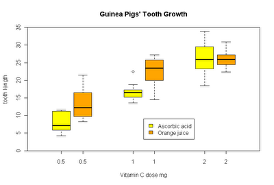
Groupwise boxplot

Groupwise boxplots can easily be created by means of the formula interface.

boxplot(len ~ supp*dose, data = ToothGrowth,
        main = "Guinea Pigs' Tooth Growth",
        xlab = "Vitamin C dose mg", ylab = "tooth length",
        col=c("yellow", "orange") 
        )

Why an outdated method is described in the boxplot help is however not directly clear. Maybe we are glad to know about the technique anyway someday...

boxplot(len ~ dose, data = ToothGrowth,
       boxwex = 0.25, at = 1:3 - 0.15,
       subset = supp == "VC", col = "yellow",
       main = "Guinea Pigs' Tooth Growth",
       xlab = "Vitamin C dose mg",
       ylab = "tooth length",
       xlim = c(0.5, 3.5), ylim = c(0, 35), yaxs = "i")

boxplot(len ~ dose, data = ToothGrowth, add = TRUE,
       boxwex = 0.25, at = 1:3 + 0.15,
       subset = supp == "OJ", col = "orange")

legend(2, 9, c("Ascorbic acid", "Orange juice"),
      fill = c("yellow", "orange"))

SQL-OLAP in R

How to generate SQL-OLAP functions in R:

d.frm <- data.frame( x=rep(1:4,3), g=gl(4,3,labels=letters[1:4]) )

# SQL-OLAP: sum() over (partition by g)
# (more than 1 grouping variables are enumerated like ave(..., g1,g2,g3, FUN=...)):
d.frm$sum_g <- ave( d.frm$x, d.frm$g, FUN=sum )


# same with rank (decreasing):
d.frm$rank_g <- ave( -d.frm$x, d.frm$g, FUN=rank )
d.frm


# get some more data
d.frm <- data.frame(
  id=c("p1","p1","p2","p2","p2","p3","p2","p3","p1","p1","p2"),
  A=c(0,1,1,1,0,0,0,0,0,0,0),
  B=c(1,0,0,0,0,0,0,0,0,0,0),
  C=c(0,0,0,0,1,1,1,0,1,1,1)
)

# get rownumber by group, based by original order
d.frm$rownr <- ave( 1:nrow(d.frm), d.frm$id, FUN=order )

# get some groupwise aggregation on more than one column 
d.frmby <- data.frame( lapply( d.frm[,-c(1,5)], tapply, d.frm$id, "max", na.rm=TRUE ))

# (see also 'Split - Apply - Combine' post)

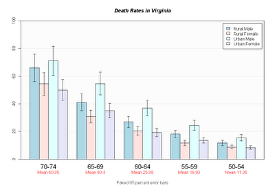
Barplot mit Fehlerbalken

hh <- t(VADeaths)[, 5:1]
ci.l <- hh * 0.85
ci.u <- hh * 1.15


mb <- barplot(hh, beside = TRUE, ylim = c(0, 100)
  , col = c("lightblue", "mistyrose","lightcyan", "lavender")
  , main = "Death Rates in Virginia", font.main = 4
  , sub = "Faked 95 percent error bars", col.sub = "gray20"
  , cex.names = 1.5
  , legend.text = colnames(VADeaths), args.legend = list( bg="white" )
  , panel.before = {
      rect( xleft=par()$usr[1], ybottom=par()$usr[3], xright=par()$usr[2], ytop=par()$usr[4]
        , col="gray99" )
      grid( nx=NA, ny=NULL ) # horiz grid only
      box()
  }
  , xpd=F )


arrows( x0=mb, y0=ci.l, y1 = ci.u, angle=90, code=3, length=0.05 )


mtext( side = 1, at = colMeans(mb), line = 2,
text = paste("Mean", formatC(colMeans(hh))), col = "red" )

Simple textplot

Putting text on a plot is not that straight on, especially if there's more than one line of text.

data(iris)

# put the summary output into a variable
out <- capture.output( 
  summary(lm(Sepal.Length ~ Species + Petal.Width, iris)) )

cat( out, sep="\n" )

# create plot
plot.new()

# print text in mono font
text(labels=out, x=0
  , y=rev(1:length(out)) * strheight( "S", cex=0.8 ) * 1.3
  , adj=c(0,0), family="mono", cex=0.8 )



This is what I thought so far. Of course it is straight on to place bulk text on several lines, stupid...
Just collapse the text with newline as separator:

text(labels=paste(out, collapse="\n"), x=0, y=0
      , adj=c(0,0), family="mono", cex=0.8 )

Format

Tausender-Trennzeichen und Nachkommastellen
format( 1234, big.mark="'", nsmall=2 )
[1] "1'234.00"


leading zeros
sprintf("%04d", 15)
[1] "0015"

oder mit formatC:
formatC(1:5, width=2, flag="0")
[1] "01" "02" "03" "04" "05"


date
format( Sys.time(), "%Y-%m-%d %H:%M:%S" )
[1] "2010-05-19 10:31:57"

numers as hexnumbers
sprintf("%1$d %1$x %1$X", 0:255)

Codes unter R-Help: strptime 

Von R zu Word

Control MS Word from R, do some reporting. The package RDCOMClient is great for that.
The library DescTools (available on CRAN) uses this package and contains some wrapping functions to make things easier.